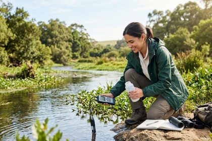
You spent years in the lab dissecting organisms, memorizing metabolic pathways, and running PCR tests. Now you are ready for the real world, but you want to apply that knowledge to something bigger: p...

You spent an hour measuring every drop of titrant, carefully noting the volume at the endpoint. Then you sit down to calculate the pH and your answer is nowhere near what the lab manual says. Or worse...
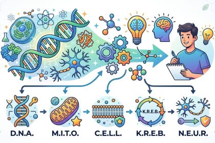
Biology demands a lot from your memory. From the stages of mitosis to the names of every bone in the hand, the sheer volume of terms can feel overwhelming. You sit down to study, review your notes, an...
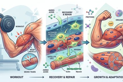
You just finished a tough set of bicep curls. Your arms feel like jelly. You look in the mirror and think, "Is anything actually happening in there?" The answer is yes. A lot. And most of it happens w...
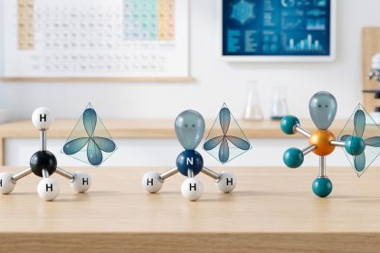
You have a molecule, and you need to know its shape. Maybe it’s for a homework assignment, maybe it’s for an exam question that’s worth a few points. Either way, staring at a chemical formula and tryi...
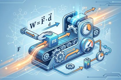
If you have ever pushed a heavy box across the floor or lifted a backpack onto a shelf, you have experienced work and power in action. But in physics, these words have very specific meanings that may ...

You’ve probably memorized the formula a² + b² = c². But when does that neat little equation actually matter outside a math worksheet? More often than you might think. From framing a house to calculati...
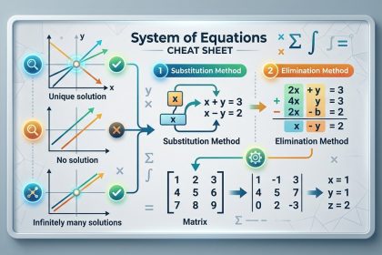
You are staring at two equations and they both have the same variables. Somewhere in that tangle of x and y lives a single point (or many points) that makes both equations true. Finding that point is ...
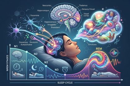
Every night, a strange and vivid movie plays inside your head. You might fly through impossible landscapes, confront forgotten faces, or wake up in a cold sweat from a monster chase. These nighttime s...
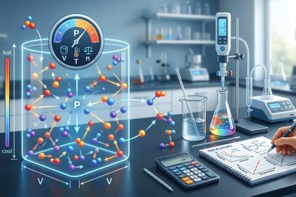
When you study gases in chemistry, one equation stands above the rest: PV = nRT. This simple formula connects pressure, volume, temperature, and amount of substance. If you can master it, you gain the...